Sunday, September 18, 2016

Deduplication and Connected Components

Consider a web application where users sign up with their email.  Some users may sign up with multiple emails and some emails may be affiliated with multiple emails.

Code Snippit:

 1
 2
 3
 4
 5
 6
 7
 8
 9
10
users = {
    tuple(['u1',]): ['e1', 'e2'],
    tuple(['u2',]): ['e1', 'e3'],
    tuple(['u3',]): ['e4'],
    tuple(['u4',]): ['e2', 'e5'],
    tuple(['u5',]): ['e6'],
    tuple(['u6',]): ['e7', 'e8'],
    tuple(['u7',]): ['e8'],
    tuple(['u8',]): ['e1', 'e9']
}

Users has a one-to-many relationship with duplications in this initial input, but our goal is to "deduplicate" this data so that we have many-to-many relationships without any loss of data.

Expected Output:

1
2
3
4
5
6
7
8
9
--((List of Deduplicated Users))--
 -- Num Users:  8
 -- Num Emails: 9
  {
     ('u2', 'u8', 'u4', 'u1'): ['e9','e5','e1','e3','e2'],
     ('u5',): ['e6'],
     ('u7', 'u6'): ['e7','e8'],
     ('u3',): ['e4']
  }

Since u1 and u2 shared e1 in common, we combined u1+u2 = e1+e2+e3.  This combined user also shared in common an e2 with u4 and an e1 with u8, so ultimately, these were deduplicated into u1+u2+u4+8 = e1+e2+e3+e5+e9.

Brute Force Approach


A brute force approach to solving this problem is as follows.  We can iteratively make changes to the list of users, compressing it by iterating over every pair of users.  In the first pass of our example, we would check u1 vs u2 for common emails.  A simple set intersection will reveal any common elements shared between the two users, so if this operator shows any comparisons, we can perform a set union of both the users and emails to get the combined u1+u2 = e1+e2+e3 as desired.  If there is no set intersection, we can be sure that the intersected users have no emails in common, and are distinct from each other -- for now.

At every intersection test, if we discover an intersection, we can append the combined user to a dedup_users data structure, which contains processed elements of our list of users.  As expected, if we combine ui+uj, we would want to delete ui and uj from the dedup_users data structure, if they exist.  In case the set union and set intersection are identical, we make sure this operation happens before we insert the combined user element into our data structure (i.e. line 10 below).


 1
 2
 3
 4
 5
 6
 7
 8
 9
10
11
if len(set(users[u]).intersection(set(users[v]))) > 0:
    try:
        del dedup_users[u]
    except:
        pass
    try:
        del dedup_users[v]
    except:
        pass
    dedup_users[tuple(list(set(u).union(set(v))))] = list(set(users[u]).union(set(users[v])))
    changes_made = True

After examining every pair in our iteration, we can reprocess the list of deduplicated users again if there were any changes made.  The running time complexity of such an algorithm is at best, O(N^2), because each pass requires examining every pair of users.  Repeated iterations would examine smaller and smaller subsets until the subset becomes the desired deduplicated results.  Another runtime analysis is to consider the use of set union and set intersection, which are both O(|u_i|+|u_j|) if i and j as the ith and jth user being compared.  This means we can say that the algorithm is generally O(N^3) if the number of emails in a user is relatively small (as it probably is).

O(N^3) is not a polynomial runtime, and increasing the size of N by a factor of 10 would increase the runtime by a factor of 10*10*10 = 1000.  For small user sets, we can show fair runtimes (0-10 seconds).  But this quickly scales out of control for say, user sets of size 100 or more.  A better algorithm is necessary if we are to expect more than 100 users.

Graph Theory Approach


Upon thinking about the problem a little closer, we can see that there are relationships between emails and users, and anytime you have relationships, you could utilize graph theory.  In our case, we would want a graph where edges between two users represent that the two users share that edge (and edges would have the attribute to indicate its email).

In its unchanged state, our list of users would need to be inverted in a sense, so that we can see all users associated with a single email.  We can do this in linear O(N) time by examining each user once, using hash tables and set theory.

1
2
3
4
5
6
7
8
9
#invert the users dictionary - O(|emails|) -> O(N)
emails = {}
for user in users:
    for email in users[user]:
        try:
            emails[email].add(user)
        except:
            emails[email] = set([user])
emails = {key: list(emails[key]) for key in emails}

With a list of 1-email to many-users, we can build our graph by iterating over pairs of users within each email.  The user pairs are the nodes, and the email is an edge.  If the user has only a single email, we can represent a trivial edge as an edge that goes out from the node and back into the node.  This would also work in O(N) time, since every user is only visited once.  To facilitate our code, we use the Network X library from Python (and have imported networkx as nx).

1
2
3
4
5
6
7
8
#build graph -- network x library - O(|emails|) -> O(N)
G = nx.Graph()
for email in emails:
    if len(emails[email]) > 1:
        for u1,u2 in zip(emails[email][:-1], emails[email][1:]):
            G.add_edge(u1, u2, email=email)
    else:
        G.add_edge(emails[email][0], emails[email][0], email=email)


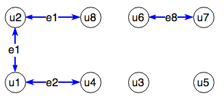
In the graph above, we omit trivial edges.  In fact the edges don't matter all that much in terms of emails, as we can always grab the emails from the list of initial users.

Lastly, we employ our coup-de-grace to wrap this problem up.  We can observe that unique user sets are disconnected from the rest of the graph.  Each of these 'groupings' are called Connected Components.  The Network X library employs an algorithm for connected components which is O(|V|+|E|) or O(|users| + |emails|), but we can call this O(N).

The output through Network X gives us a list of lists, where each list is a connected component containing a list of users in that group.  For instance, the result on our graph here would be [[u1,u2,u4,u8], [u3], [u5], [u6,u7]].  This also gives us lists of deduplicated users, but we just have to get the emails to go with them!  This leads us to our final step -- again, using set theory to union together groups of emails associated with each user in our connected components.

 1
 2
 3
 4
 5
 6
 7
 8
 9
10
dedup_users = {}
ccs = nx.connected_components(G) #O(V+E) -> O(N)

#O(N) -- every user is hit only once.  Add  complexity of set unions
for cc in ccs:
    user_list = tuple([c[0] for c in cc])
    email_list = set()
    for user in user_list:
        email_list = email_list.union(set(list(users[tuple([user])]))) # -> O(|users[user]|)
    dedup_users[user_list] = tuple(list(email_list))

Finally, we can simply return the list of deduplicated users for evaluation and assurance of correctness.  Overall, this graph theory approach can be described generally as O(N) * O(|connected components|).  Since the number of connected components can equal as high as N in the case where every single user is perfectly distinct, this algorithm has a worst case of being O(N^2).  When you think about it, it's more likely that a majority of the users are "normal" in the sense of registering only a single email each, so the average case is probably closer to O(N^2).

Utility Functions

To test and assert the correctness of our two algorithms -- Brute Force and Graph Theory, we built some utility functions.  First, we built a pretty printer so that we can visually output our user dictionaries and appropriately eye the correctness as the code was being implemented.  This helped visually identify bugs and get to a working solution.


 1
 2
 3
 4
 5
 6
 7
 8
 9
10
11
12
13
14
15
16
17
18
19
20
21
22
23
24
25
26
27
28
29
30
31
32
33
34
35
36
37
38
39
40
41
42
43
44
45
def pretty_print_dict(users):
    """Pretty prints a dictionary of users
       :param: users is a dictionary to pretty print

       returns None
    """

    max_n = 10
    cur_n = 0
    len_n = len(users)

    max_e = 5
    max_u = 5

    s = ""
    s += "  {\n"

    for user in users:
        if (cur_n < max_n and cur_n < len_n):
            cur_n += 1
            if len(user) < max_u:
                s += "     " + str(user) + ": "
            else:
                s += "      (" + ','.join(["'" + str(u) + "'" for u in list(user)][:max_u]) + " + " + str(len(user)-max_u) + " more...)" + ": "

            s += "["
            cur_e = 0
            len_e = len(users[user])
            for e in users[user]:
                if (cur_e < max_e and cur_e < len_e):
                    cur_e += 1
                    s += "'" + str(e) + "'" + ","
                else:
                    break
            if cur_e < len_e:
                s += " + " + str(len_e - cur_e) + " more,"
            s = s[:-1]
            s += "],\n"
        else:
            break
    if cur_n < len_n:
        s += "     < ... " + str(len_n - cur_n) + " more keys>,\n"
    s = s[:-2] + "\n"
    s += "  }"
    print s


Secondly, we built an evaluator that would assert the correctness of the finalized results.  This check involved three things: 1) did we lose any emails?  2) did we lose any users?  and 3) are the users and emails listed exactly once each?


 1
 2
 3
 4
 5
 6
 7
 8
 9
10
11
12
13
14
15
16
17
18
19
20
21
22
23
24
25
26
27
28
29
30
31
32
33
34
35
36
37
38
39
40
41
42
43
44
45
46
47
def assert_correctness(users, correct_num_users, correct_num_emails):
    """Assert the correctness of the deduplication process
       :param: users is the deduplicated dictionary of users to assert correctness
       :param: correct_num_users is the expected number of unique users
       :param: correct_num_emails is the expected number of unique emails

       returns None -- output result is printed here instead

       Explanation: A dictionary of users is deduplicated if the set of unique users and emails found throughout
       the dictionary amount to the same amount of users we started with.  This ensures we did not lose any information.
       Second, we require that no email found in any user is found in any other user.  This ensures that the dupication
       clause is correct.
    """

    #Test of the Loss of Data Clause
    set_users = set([])
    set_emails = set([])
    for key in users:
        for item in key:
            set_users.add(item)
        for val in users[key]:
            set_emails.add(val)


    #Test the duplication clause
    violations_found = 0
    already_probed = {}
    for user in users:
        for other_user in users:
            if not user == other_user and not already_probed.get((user, other_user), False):
                already_probed[(user,other_user)] = True
                if len(set(list(users[user])).intersection(set(list(users[other_user])))) > 0:
                    violations_found += 1


    #Pretty print deduplicated users
    print "\n--((List of Deduplicated Users))--"
    print " -- Num Users:  " + str(len(set_users))
    print " -- Num Emails: " + str(len(set_emails))
    pretty_print_dict(users)


    #Print out report
    print "\n--((Assertion Evaluation))--"
    print " -- Users look unique and correct!" if len(set_users) == correct_num_users else " -- These users don't look right."
    print " -- Emails look unique and correct!" if len(set_emails) == correct_num_emails else " -- These emails don't look right."
    print " -- Duplication Violations found: " + str(violations_found)


Thirdly, we wanted to test our algorithm on a variety of unbiased inputs, so we build a random generator that would construct random user and email sets.  This generator takes a few inputs, namely the number of users to generate and a probability function that describes the odds of having 1 - E emails in each user.  Additionally, a variety parameter was used to control the rate of collision of users having duplicated emails.


 1
 2
 3
 4
 5
 6
 7
 8
 9
10
11
12
13
14
15
16
17
18
19
20
21
22
23
24
25
26
27
28
def gen_random_users(N = 10, tiers = [0.70, 0.80, 0.90, 0.95, 0.98, 0.99, 0.999], V = 1):
    """generates a random dictionary of users and emails
       :param: N controls the number of users to be generated
       :param: tiers controls the probabilities of increasing numbers of emails per user
       :param: V controls the variety of the emails generated.  Higher V = less chance of duplicate

       returns users - a list of random users with random emails
    """

    users = {}
    set_emails = set([])
    variety = V*N/10
    for i in range(1,N+1):
        #gen random list of emails
        f = random.random()
        for t,tier in enumerate(tiers):
            if f < tier:
                n = t+1
                break
        emails = []
        for j in range(n):
            emails.append(random.randint(1,10+variety))
        emails = list(set(emails))
        emails = ['e'+str(e) for e in emails]
        for email in emails:
            set_emails.add(email)
        users[tuple(['u'+str(i),])] = emails
    return users, N, len(set_emails)


Comparing Brute Force to Graph Theory


Our Brute Force algorithm is O(N^3) and the Graph Theory approach is O(N^2).  Our Graph Theory approach should be much faster, right?  Indeed.  When run on the same set of users, we can see dramatic speeds.  For larger N, these speedups would be even faster.

For one random case of 10 users, our Brute Force approach took 2.149 seconds, while our Graph Theory approach took 0.001 seconds, indicating a speedup of over 2000x.  This greatly varies, since our two algorithms have different strong and weak points.

For 50 users, it is generally very difficult for the Brute Force approach to work in any bearable amount of time, while the Graph Theory approach can run in mere fractions of a second.  I was able to see bearable runtimes up to N=50000 in about 9 seconds, but when we tweak the random generator so that most emails are never duplicated, the runtime for Graph Theory approach increases, and N=2000 would run in about 4 seconds (yet still, at large N, Graph Theory approach would win over Brute Force in any situation).

Connected Components


For details on connected components, refer to https://en.wikipedia.org/wiki/Connected_component_(graph_theory) for an overview.  The general essence of any algorithm for obtaining connected components is to perform a Depth-First-Search on the graph, traversing and visiting nodes, making notes of when you need to "lift your pen" to hop to another connected component of the graph.

A similar application, Strongly Connected Components, occurs only in directed graphs.  In our application, we utilized general undirected graphs, so any node within a connected component could be reached from any other node in the same connected component.  With directed graphs, we encounter situations where we may not be able to return to a node once we left it.  One algorithm for solving the problem of strongly connected components is Tarjan's Algorithm.  The general idea here, is that any cycle or a single vertex is a strongly connected component.


Full Source Code


This code was implemented using Python 2.7.6 and Network X 1.9.1.
Source code available here: http://pastebin.com/gKxYuEHC

Tuesday, September 13, 2016

Week of Code - Sorting Algorithms

The topic of Sorting Algorithms is a very key subject within computer science algorithms study, as it is often frequently used in much larger coding projects.  There are a number of well-known algorithms, such as Merge Sort, Quick Sort, Insertion Sort and Bubble Sort, which should be well-studied by the avid computer scientist.  Before one could properly analyze each, we need to assume an understanding of Big-O Notation and algorithmic complexity analysis.

In this blog post, we look at some of these popular sorting algorithms and implement them in Python.  I've set up a way to benchmark the speeds of each and verify their correctness, and we will be able to see how they perform under different characteristics.


Bubble Sort

We start with perhaps the most trivial sorting algorithm - the Bubble Sort.

1
2
3
4
5
6
7
8
def bubbleSort(arr):
    larr = len(arr)
    for i in np.arange(larr):
        for j in np.arange(larr - i - 1):
            if arr[j] > arr[j+1]:
                temp = arr[j+1]
                arr[j+1] = arr[j]
                arr[j] = temp

This algorithm essentially iterates over the array from left to right.  At each item, it then searches for an item to the right of it that it needs to swap.  After passing through each item in this manner, it follows that all of the items will be ordered properly.

The outer loop will always run n-many times.  The inner loop varies from running one time during each pass (the best case), or n-i many times times in each pass (the worst case).  One exercise is to consider when these cases happen.  For instance, when the list is in reverse order, we can expect the worst case.  The best case on the other hand, will happen when the list is already nearly sorted.

It follows that the the worst case of Bubble Sort is O(N²), but its best case can be O(N).  A python implementation above shows best-of-5 runtimes for Bubble Short as follows.  Every time the size of the list increased ten-fold, the runtime increased one-hundred-fold.  For mostly sorted lists, the runtime was about 33% faster.

Indeed, some argue that Bubble Sort isn't even worthwhile to teach others, due to how fast it scales in runtime as the size of the sorting list grows.  However, I argue that the simplicity of the sort offers an incubational problem solving environment to many who wish to begin studying algorithms.

Mostly Sorted? N Runtime (s)
No 10 0.00012
Yes 10 0.00011
No 100 0.00349
Yes 100 0.00227
No 1000 0.32612
Yes 1000 0.20100
No 10000 33.4892
Yes 10000 20.6090


Insertion Sort

The Insertion Sort, like Bubble Sort, is not a very fast sort although it is still a relatively simple sorting algorithm.  While it remains of the same class of algorithms as Bubble Sort, the Insertion Sort has a much faster potential if the list is already mostly sorted.

1
2
3
4
5
6
7
8
def insertionSort(arr):
    for i in np.arange(1, len(arr)):
        currentvalue = arr[i]
        position = i
        while position > 0 and arr[position-1] > currentvalue:
            arr[position] = arr[position-1]
            position = position-1
        arr[position] = currentvalue

Ultimately, the insertion sort will still iterate over each element once in the outer loop.  It then makes a note of the index at that location, and then begins to iterate backwards looking for inversions that need to be corrected by inserting the out-of-order element before the indexed position.

One other way to understand this algorithm is to consider a hand of cards that you need to sort.  Typically, you'd look at the first card, and then scan right of it looking for any cards smaller than it, and you'd insert those before your first card in sorted order.

At its worst case, the Insertion sort requires N passes of the outer loop and N-i passes of the inner loop, which could happen if the list was reverse-sorted.  This is O(N²) at worst case, but O(N) at its best case.  This sounds identical to Bubble Sort, but why is Insertion Sort faster than Bubble Sort at its best case?  The code for our Insertion Sort can utilize a While loop in its inner loop, whereas the Bubble Sort used a For loop.  In the best case for Bubble Sort, it still had to iterate over N-i items in every inner loop.  However, the Insertion Sort code can opt out of its Inner While loop at any time, and on the very first pass of best cases.

The runtime analyses still demonstrates the scale of quadratic complexity.  Every time N increases by one order of magnitude, the runtime increased by two orders of magnitude.  It's worth noting that in practice, people tend to sort lists that are already sorted, meaning that the "mostly sorted" case is more frequent than a totally random list.  This is a good feature of Insertion Sort, but as we will see, there are far better sorting algorithms.

Mostly Sorted? N Runtime (s)
No 10 0.00003
Yes 10 0.00003
No 100 0.00213
Yes 100 0.00029
No 1000 0.20506
Yes 1000 0.02768
No 10000 20.7122
Yes 10000 2.39983


Merge Sort

The Merge Sort is one of our more complex algorithms, and more generally, a Divide-and-Conquer algorithm.  Using recursion, the problem size is divided into most basic elements (lists of size 1), and then they are "conquered" by recombining them into a sorted parts, and then finally into a sorted whole.

 1
 2
 3
 4
 5
 6
 7
 8
 9
10
11
12
13
14
15
16
17
18
19
20
21
22
23
24
25
26
27
28
29
30
31
32
33
34
35
36
37
38
39
40
41
def mergeSortLen(part):
    """takes an unsorted list and returns a sorted list
    """

    if len(part) > 1:
        mid = len(part)/2
        left = mergeSortLen(part[:mid])
        right = mergeSortLen(part[mid:])

        i = 0
        j = 0
        k = 0

        llen = len(left)
        rlen = len(right)
        while i < llen and j < rlen:
            if left[i] > right[j]:
                part[k] = right[j]
                j += 1
            else:
                part[k] = left[i]
                i += 1
            k += 1

        if i < j:
            remaining = left
            remlen = llen
            r = i
        else:
            remaining = right
            remlen = rlen
            r = j

        while r < remlen:
            part[k] = remaining[r]
            r += 1
            k += 1

        return part
    else:
        return part

The source code for Merge Sort is much more complex than Insertion Sort or Bubble Sort, but the pay-off is worth it.  An understanding of Merge Sort assumes an understanding of basic Recursion.  That is, the code will call itself on a smaller part of the input until the input becomes so small it matches the recursive base case, at which point it no longer calls itself, but proceeds to reconstruct the pieces in a sorted fashion.

Consider an unsorted list:

374591

This would first be split (as into a leaf and leaf nodes) into:
374     and     591

Which then would further keep splitting:
       3   &   74    and      5  &  91
                7  & 4                    9 & 1

Once the tree has been split into each of its leaf nodes, we can then begin reconstructing the list by marrying leaf nodes with its direct sibling node.   Our lowest two pairs of sibling-pair leaf nodes are "7 & 4" and  "9 & 1".   These are both inverted, so the reconstruction would swap them into "4 & 7" and "1 & 9".

At this point, our recombination would need to marry "3 & 47" and also marry "5 & 19".  The sorting technique here is to place pointers on both sides.  At each step, we compare two elements, selecting the smaller of the two to be placed into the joined list.  For instance, with "3 & 47", we'd compare 3 vs 4, selecting the 3 to go into the first spot of the joined list.   And then we'd pick the 4, and then the 7, so we'd have a joined list of "347".   For "5 & 19", we'd have to pick 1 first, and then the 5 and 9.

This gives us a tree which looks like:
347    and    159

One final recombination step initializes pointers at the 3 and 1.   Since 1 is smaller, we select it first, which advances the right-side pointer to the 5, so that we are comparing 3 vs 5.  Pick the 3, and then we're comparing 4 vs 5, and so on.  The final combination gives us our final sorted list of 134579.

In our code, it is possible that our pointers exhaust one of the two sides before it exhausts the other.  in this case, we have to handle remaining elements and sort them in a similar fashion.

The analysis of Merge Sort could be solved with Recurrence Relations.  There are two recursive calls which operate on half of the input, and then there is a linear O(N) section that follows the recursive calls to recombine the pieces.  Hence, T(N) = 2T(N/2) + O(N), which is of the form, aT(N/b) + f(N), and we can use the Master Theorem's case two to show that T(N) = O(N log N), and that the best case and worst case are the same.

The runtime of Merge Sort can vary greatly on its actual implementation.  In our code, we utilize the len() method as little as possible to achieve a fairly minimal runtime.  For a list with 10000 elements, we can see that the runtime is about 500 times faster than Bubble Sort, and even ~33 times faster than Insertion Sort in its best case.  We can also see that Merge Sort has very little variance in the runtimes between mostly sorted lists and totally random lists, which follows from the fact that its best and worst cases are of the same complexity.

Mostly Sorted? N Runtime (s)
No 10 0.00003
Yes 10 0.00003
No 100 0.00058
Yes 100 0.00055
No 1000 0.00643
Yes 1000 0.00496
No 10000 0.06727
Yes 10000 0.06211


Quick Sort

Like Merge Sort, the Quick Sort is a recursive Divide-and-Conquer function.  Its primary difference is that it relies on the selection of a pivot to decide on how to split the parts into two.  After the parts are split, the "conquering" recombination portion of the code is moot, because all that is needed is to recombine the pieces as each side will be ready to marry in perfect sort order.

 1
 2
 3
 4
 5
 6
 7
 8
 9
10
11
12
13
14
15
16
17
18
19
20
21
def quicksort(arr):
    quicksorthelper(arr, 0, len(arr)-1)

def quicksorthelper(arr, first, last):
    if first < last:
        pivot = partition(arr, first, last)
        quicksorthelper(arr, first, pivot-1)
        quicksorthelper(arr, pivot+1, last)

def partition(arr, first, last) :
    pivot = last
    swap(arr, pivot, last)
    for i in np.arange(first, last):
        if arr[i] <= arr[last]:
            swap(arr, i, first)
            first += 1
    swap(arr, first, last)
    return first

def swap(A, x, y):
  A[x],A[y]=A[y],A[x]

The selection of a pivot for Quick Sort is a big topic.  In general, three easy choices can be either the first element, the last element or the middle element.  In this source code, we select the last element, because it is known that Quick Sort can be slow if it chooses the first element on an already sorted list.

Quick Sort works as follows.  After selection of a pivot, the list is divided into the section to the left and right of the pivot (of its value, not index).  The elements of each side are then recursively sorted in the same way.  The recombination step has nothing to do, since the pivot partition was done in such a way that elements greater than the pivot were moved into the right side, and elements less than the pivot are moved into the left side.

Asymptotically, Quick Sort is in the average case, an O(N log N) algorithm, however its worst case can be O(N²).  This can happen in the case of an unbalanced splitting of the list, e.g. one side has all of the elements on every split.  This can make the selection of the pivot a very important factor.  The reason the first element is often a poor choice is because in practice, lists are usually already sorted or mostly sorted, which can lead to poor performance behavior.

Indeed, we see that for mostly-sorted lists, Quick Sort performs much worse.  However, it is still far faster than Bubble Sort and Insertion Sort.  Compared to Merge Sort, there is basically no difference except for its mostly-sorted case.

Mostly Sorted? N Runtime (s)
No 10 0.00002
Yes 10 0.00005
No 100 0.00036
Yes 100 0.00084
No 1000 0.00559
Yes 1000 0.01608
No 10000 0.06909
Yes 10000 0.16705


Tim Sort

So far, we could argue that Merge Sort is a clear winner of all algorithms shown so far.  How could one make Merge Sort faster?  Python's native sorting algorithm is one called Tim Sort, which is a hybrid algorithm that combines features of both the Merge Sort and Insertion Sort.  We have seen that Insertion Sort performs very well on mostly-already sorted sequences.  In Tim Sort, the algorithm finds subsequences of mostly-sorted data and exploits those regions to more efficiently sort the remaining portions.

1
2
def timsort(arr):
    arr.sort()

The source code for using Tim Sort is basically to just call the sort() method on any list data that can be sorted.  We use a wrapper to bring benchmarks on the sorting algorithm for comparison with the others.

As we can see, the runtimes for Tim Sort are improved with mostly-sorted lists, and even in its slower cases, it is about 20 times faster than even Merge Sort, and up to 40 times faster for already-sorted lists.   Asymptotically, Tim Sort is worst case O(N log N) and best case of O(N), making Tim Sort a linear algorithm at best.

Mostly Sorted? N Runtime (s)
No 10 0
Yes 10 0
No 100 0.00002
Yes 100 0.00001
No 1000 0.00027
Yes 1000 0.00015
No 10000 0.00369
Yes 10000 0.00154


Utility Source Code

We used a random list generator that used Numpy.  To ensure sparsity of the generated random numbers, we make the range of numbers to generate much bigger than the number of elements that is needed.  To generate mostly sorted lists, we took 5% of the elements and inverted them randomly.

To ensure the correctness of our algorithms, we ran them through a verify_correct() method which iterates over every subsequent pair of elements to ensure that they were ordered properly.

Our benchmark tool ran for N = 10, 100, 1000 and 10000 elements, and for both randomized lists and slightly-out-of-order lists.  For each level of N and orderliness, we ran the sorting algorithm 5 times and chose the best runtime (best-of-five), meaning that every sorting algorithm ran 5*4*2 = 40 times.

 1
 2
 3
 4
 5
 6
 7
 8
 9
10
11
12
13
14
15
16
17
18
19
20
21
22
23
24
25
26
27
28
29
30
31
32
33
34
35
36
37
38
39
40
41
42
43
44
45
46
47
48
49
50
51
52
53
54
55
56
57
def genRandomList(n = 21, neatness = 0.50, sparsity=20):
    return list(np.random.randint(low=-n*sparsity, high=n*sparsity, size=n))

def genMostlySortedList(n = 21, neatness = 0.50, sparsity=20):
    arr = list(np.random.randint(low=-n*sparsity, high=n*sparsity, size=n))
    arr.sort()
    f = 0.05
    larr = len(arr)
    for i in range(int(f * larr) + 1):
        x = random.randint(0, larr-1)
        y = random.randint(0, larr-1)
        temp = arr[x]
        arr[x] = arr[y]
        arr[y] = temp
    return arr

def verify_correct(arr):
    for item,next in zip(arr[:-1], arr[1:]):
        if item <= next:
            continue
        else:
            return False
    return True


def benchmark(method):

    for n in [10, 100]:#, 1000, 10000]:
        best_runtime = None
        correctness = True
        for repeat in range(5):
            x = genRandomList(n=n)
            time_of_start = time.time()
            method(x)
            time_of_end = time.time()
            if best_runtime is None:
                best_runtime = time_of_end - time_of_start
            else:
                best_runtime = min(best_runtime, time_of_end - time_of_start)
            correctness = correctness and verify_correct(x)
        print "{:<20s}".format(str(method.__name__)) + ", " + "mostly sorted=False" + ", " + "{:<8s}".format(str(n)) + ", " + str("%.5f" % (best_runtime)) + ", " + str("correct" if correctness else "incorrect")

        best_runtime = None
        correctness = True
        for repeat in range(5):
            x = genMostlySortedList(n=n)
            time_of_start = time.time()
            method(x)
            time_of_end = time.time()
            if best_runtime is None:
                best_runtime = time_of_end - time_of_start
            else:
                best_runtime = min(best_runtime, time_of_end - time_of_start)
            correctness = correctness and verify_correct(x)
        print "{:<20s}".format(str(method.__name__)) + ", " + "mostly sorted=True " + ", " + "{:<8s}".format(str(n)) + ", " + str("%.5f" % (best_runtime)) + ", " + str("correct" if correctness else "incorrect")

    print "-----------------------------------------------------------"


Test Driver

Finally, to run our code, we ran the benchmark() method on each of our sorting algorithms, passing along the function call of each method to be benchmarked.  The result is a print-out of the performance of each algorithm.

1
2
3
4
5
benchmark(mergeSortLen)
benchmark(timsort)
benchmark(quicksort)
benchmark(insertionSort)
benchmark(bubbleSort)


Full Code

The full code was written with Python 2.7.8 and Numpy 1.9.0.
Code available at: http://pastebin.com/YwY5K404